Use Excel CHOOSE Function to Replace Nested IFs

 

Use Excel CHOOSE Function to Replace Nested IFs

1.1 Return Value Based on Conditions

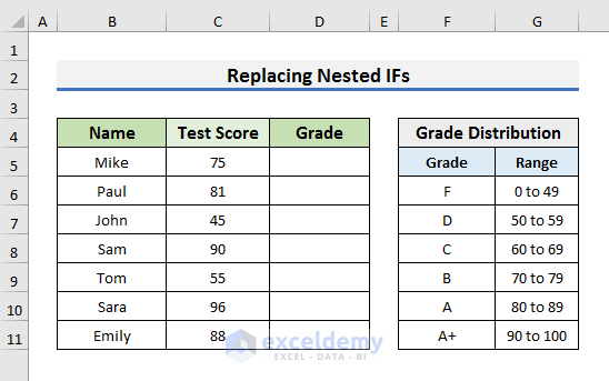
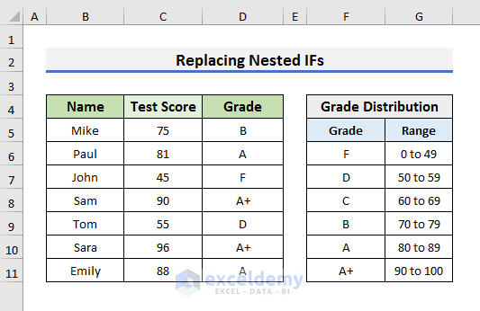
In the first case, we will return a value based on some conditions using the CHOOSE function. The dataset we will use here contains the Test Scores of some students. We can easily assign the grades using the CHOOSE function. You can see the Grade Distribution in the picture below.

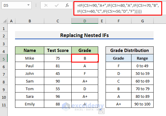
Generally, we use the Nested IFs to solve this type of problem. But Nested IFs can be confusing sometimes and may encounter problems if the equation becomes large. The Nested IFs formula for assigning the grades can be written as below:

=IF(C5>=90,"A+",IF(C5>=80,"A",IF(C5>=70,"B",IF(C5>=60,"C",IF(C5>=50,"D","F")))))

Let’s follow the steps below to see how we can use the CHOOSE function to replace the Nested IFs formula.

STEPS:

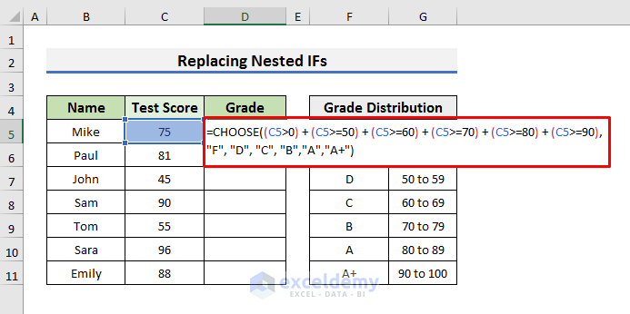
• First of all, select Cell D5 and type the formula below:

=CHOOSE((C5>0)+(C5>=50)+(C5>=60)+(C5>=70)+(C5>=80)+(C5>=90),"F","D","C","B","A","A+")

🔎 How Does the Formula Work?

• (C5>0)+(C5>=50)+(C5>=60)+(C5>=70)+(C5>=80)+(C5>=90): In this part of the formula, we have used the Grade Distribution as the index number inside the CHOOSE function. As there are multiple index numbers based on the situation, we have used the plus (+) operator to make an OR operation.
• “F”,”D”,”C”,”B”,”A”,”A+”: This part contains the values corresponding to the index numbers. Depending on the index number, the CHOOSE function will return the grades. For example, if the matched index number is between 80 to 89, then it will print “A”.

• Secondly, press Enter and drag the Fill Handle down.

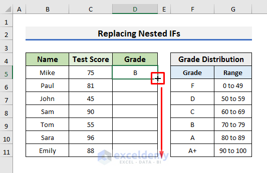
• Finally, you will be able to assign the grades based on the test scores.

1.2 Return Calculation Based on Criteria

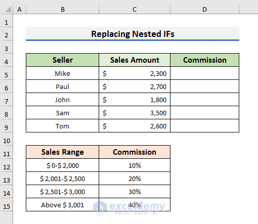
In the previous example, we returned a value based on some conditions. Similarly, we can also return the result of a calculation using the CHOOSE function. To explain the application, we will use a dataset that contains the Sales Amount of some Sellers. We will extract the Commission for each seller. You can also see the Sales Range with the corresponding percentage of Commission. For example, if the sales amount of a seller is between $2,001-$2,500, then he will get a 20% commission. We will try to find the amount of the Commission.

STEPS:

• In the first place, select Cell D5 and type the formula below:

=CHOOSE((C5>=0)+(C5>=2001)+(C5>=2501)+(C5>=3001),C5*0.1,C5*0.2,C5*0.3,C5*0.4)

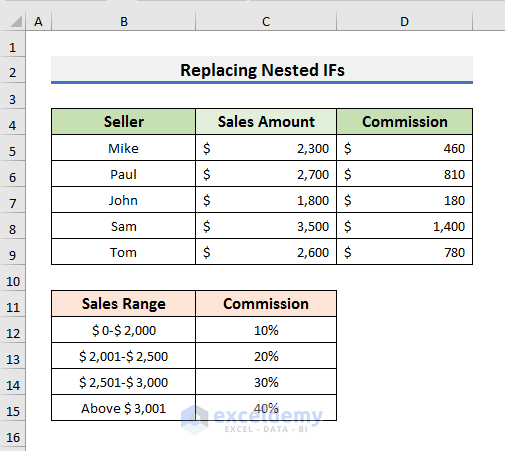
This formula is similar to the previous one. But it multiplies the value of Cell C5 with the Commission Percentage based on the index number and then returns the result.

• After that, press Enter and drag down the Fill Handle to see the commission for each seller.

https://www.exceldemy.com/