Introduction to Excel CHOOSE Function
In Microsoft Excel, the CHOOSE function selects a value or performs an action from a list of values, based on the index number. It needs two required arguments to function.
- Syntax
CHOOSE(index_num, value1, [value2]….)
- Arguments
index_num: It is the position number of the values. Position of value1 is 1, value2 is 2, and so on.
value1: It is the second required argument inside the CHOOSE function. You can enter value2, value3, and many more for your purposes.
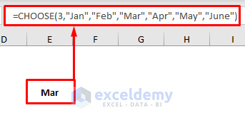
For example, if you type =CHOOSE(3,"Jan","Feb","Mar","Apr","May","June") in a cell, and, press Enter, then the output will be Mar because Mar is the third value among the specified values.
9 Advanced & Useful Applications of CHOOSE Function in Excel
In the following section, we will explain 9 advanced and useful applications of the CHOOSE function. To explain the applications, we will use different datasets. We will introduce the datasets while explaining the examples. So, let’s follow the examples below to learn more.
1. Use Excel CHOOSE Function to Replace Nested IFs
One of the most advanced and useful applications of the CHOOSE function in Excel is that you can use it to replace Nested IFs. Generally, when we have multiple criteria or conditions, we use the Nested IFs formula. We can use the CHOOSE function for the same purpose. Here, we can return a value or a calculation based on conditions. We will demonstrate both in the following subsections.
1.1 Return Value Based on Conditions
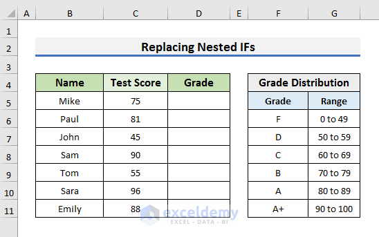
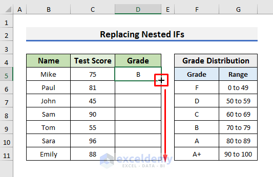
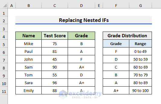
In the first case, we will return a value based on some conditions using the CHOOSE function. The dataset we will use here contains the Test Scores of some students. We can easily assign the grades using the CHOOSE function. You can see the Grade Distribution in the picture below.
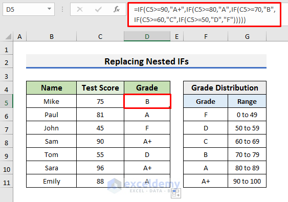
Generally, we use the Nested IFs to solve this type of problem. But Nested IFs can be confusing sometimes and may encounter problems if the equation becomes large. The Nested IFs formula for assigning the grades can be written as below:
Let’s follow the steps below to see how we can use the CHOOSE function to replace the Nested IFs formula.
STEPS:
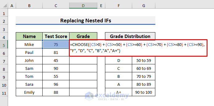
- First of all, select Cell D5 and type the formula below:
🔎 How Does the Formula Work?
- (C5>0)+(C5>=50)+(C5>=60)+(C5>=70)+(C5>=80)+(C5>=90): In this part of the formula, we have used the Grade Distribution as the index number inside the CHOOSE function. As there are multiple index numbers based on the situation, we have used the plus (+) operator to make an OR operation.
- “F”,”D”,”C”,”B”,”A”,”A+”: This part contains the values corresponding to the index numbers. Depending on the index number, the CHOOSE function will return the grades. For example, if the matched index number is between 80 to 89, then it will print “A”.
- Secondly, press Enter and drag the Fill Handle down.
- Finally, you will be able to assign the grades based on the test scores.
1.2 Return Calculation Based on Criteria
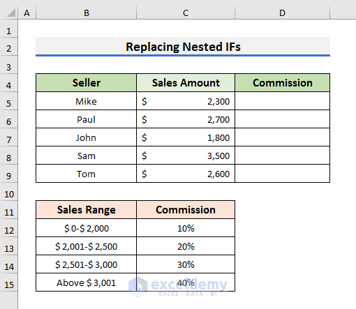
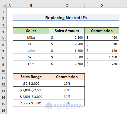
In the previous example, we returned a value based on some conditions. Similarly, we can also return the result of a calculation using the CHOOSE function. To explain the application, we will use a dataset that contains the Sales Amount of some Sellers. We will extract the Commission for each seller. You can also see the Sales Range with the corresponding percentage of Commission. For example, if the sales amount of a seller is between $2,001-$2,500, then he will get a 20% commission. We will try to find the amount of the Commission.
STEPS:
- In the first place, select Cell D5 and type the formula below:

This formula is similar to the previous one. But it multiplies the value of Cell C5 with the Commission Percentage based on the index number and then returns the result.
- After that, press Enter and drag down the Fill Handle to see the commission for each seller.
Read More: How to Use CHOOSE Function to Perform IF Condition in Excel
2. Apply CHOOSE Function for Left VLOOKUP in Excel
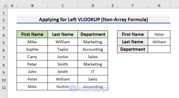
In Excel, the VLOOKUP function looks for a value in the leftmost column of a table and then returns a value in the same row from a column you specify. But in case of multiple criteria, we can’t use the VLOOKUP normally. We use the CHOOSE function with the VLOOKUP function to extract certain values based on multiple criteria. This is another advanced use of the CHOOSE function in Excel. Here, we will see the non-array and array formulas for the VLOOKUP with CHOOSE functions.
To explain both formulas, we will use a dataset that contains the First Name and Last Name of some employees. We will extract the Department based on the names.
2.1 Non-Array Formula
In the first subsection, we will use a non-array formula with the VLOOKUP and CHOOSE functions. If we use a Helper column and use it to constitute a formula, then it will make a non-array formula. Let’s follow the steps to learn more.
STEPS:
- Firstly, we need to insert a Helper column on the leftmost side. In our case, Column B is the Helper column.
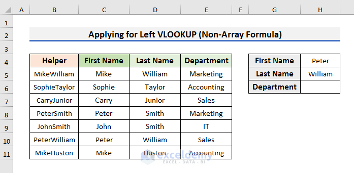
- Now, we need to concatenate the First and Last To do so, select Cell B5 and type the formula below:
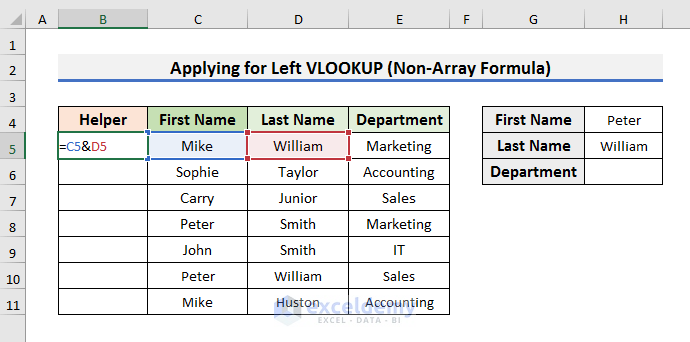
- Press Enter and drag the Fill Handle down.
- After that, select Cell H6 and type the formula below:
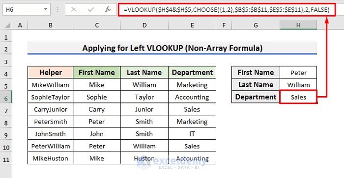
Here, the CHOOSE function creates a lookup table with Columns B & C. In this formula, the VLOOKUP function looks for the PeterWilliam value in Column B and returns the corresponding value from the lookup table that the CHOOSE function creates.
Read More: How to Use VLOOKUP with CHOOSE Function in Excel
2.2 Array Formula
If we don’t use any helper column in the case of the VLOOKUP function, then the formula becomes an array formula. We can solve the previous example with an array formula. Let’s follow the steps below for more.
STEPS:
- In the beginning, select Cell G6 and type the formula below:
- After typing the formula, press Ctrl + Shift + Enter to see the result.
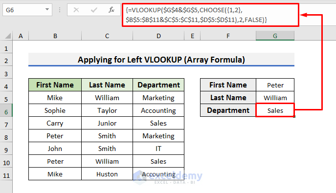
This is an array formula. It looks for the concatenated value of Cell G4 and Cell G5 in the lookup table. This time the CHOOSE function creates a lookup table of two columns. The first column concatenates the value of the range B5:B11 and C5:C11 and the second column stores the Department names. Depending on the First and Last names, it returns the Department name.
Read More: How to Use CHOOSE Function with Array in Excel
3. Insert Excel CHOOSE Function to Find Sum of Selected Variables
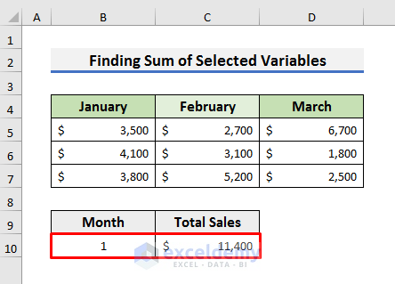
The application of the CHOOSE function inside the SUM function is very interesting. We can find the total sales of a month dynamically using the CHOOSE function. To explain this example, we will use a dataset that contains the sales amount of a seller for the first three months. We will find the total sales amount for a month in Cell C10.
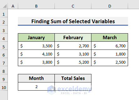
Let’s follow the steps below to learn how we can use the CHOOSE function to find the sum of selected variables.
STEPS:
- First, select Cell C10 and type the formula below:
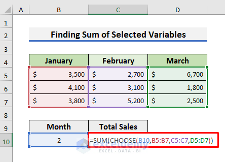
In this formula, the CHOOSE function selects the range based on the month number that we insert in Cell B10. If we enter 2 in Cell B10, then the formula becomes:
=SUM(CHOOSE(2,B5:B7,C5:C7,D5:D7))
After that, the CHOOSE function returns the range C5:C7 based on the index number.
So, finally, the formula acts as:
=SUM(C5:C7)
That is how we get the total sales for the selected month.
- Hit the Enter key to see the total sales for February.
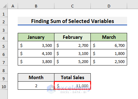
- To see the total sales for January, type 1 in Cell B10.
4. Assign Day/Month/Quarters to Dates Using Excel CHOOSE Function
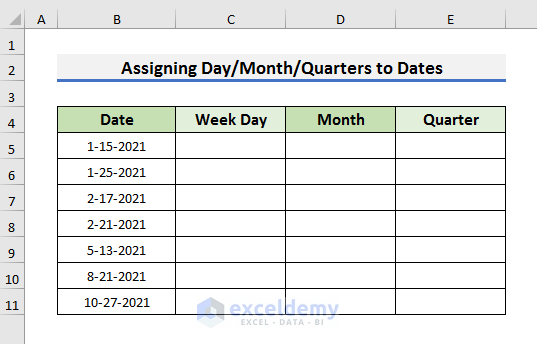
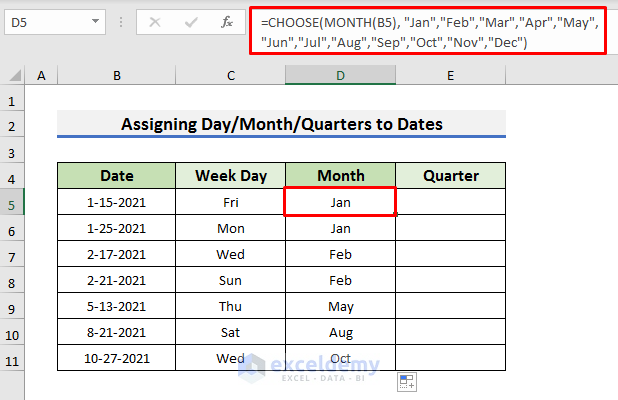
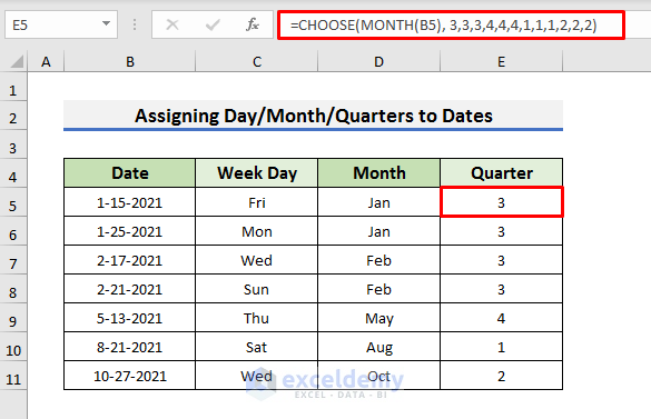
Assigning day/month/quarters to dates is another feature of the CHOOSE function. For that purpose, we need the help of the WEEKDAY function. In the dataset below, you can see the dates of some events. We will try to extract the Week Day, Month, and Fiscal Quarters from them.
Let’s pay attention to the steps below to know more about assigning weekdays, months, and quarters to dates.
STEPS:
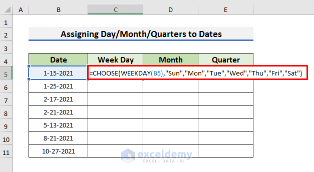
- In the first place, select Cell C5 and type the formula below to assign weekdays to dates:
Here, the WEEKDAY function returns the index number for the CHOOSE function.
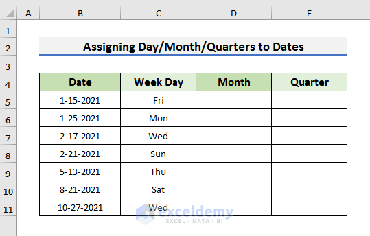
- Press Enter and drag the Fill Handle down to see weekdays for all dates.
- Similarly, to assign months to dates, use the formula below in Cell D6:
In this formula, the MONTH function finds the month number and uses it as the index number.
- Finally, for Fiscal Quarters, you can use the formula below:
5. Use CHOOSE Function to Return Value Based on Index Number
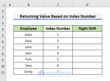
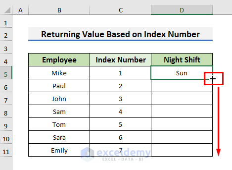
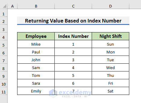
This is a basic application of the CHOOSE function. Generally, it returns a value from the list based on the index number. The index number is the first argument of the CHOOSE function. In the dataset below, we have some employees with index numbers. Using the index numbers, we will assign the weekdays for night shifts.
Let’s observe the steps below to learn more about the example.
STEPS:
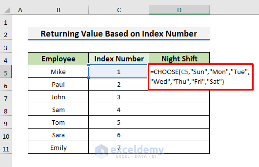
- First, select Cell D5 and type the formula below:
In this formula, Cell C5 contains the index number, and based on the index number, the CHOOSE function returns a weekday for the night shift.
- After that, press Enter and drag the Fill Handle down.
- Finally, you will be able to return a value based on the index number.
6. Apply CHOOSE Function for Reverse VLOOKUP in Excel
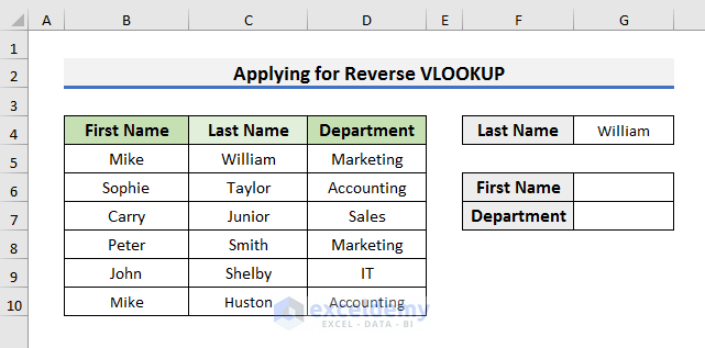
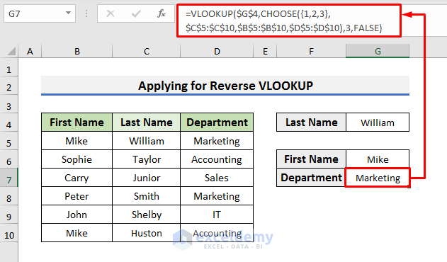
Usually, the VLOOKUP function looks for a value in the leftmost column. But with the help of the CHOOSE function, we can make the VLOOKUP look for a value in other columns. This can be called the reverse VLOOKUP in Excel. For explaining the example, we will use the dataset of Example 2. But this time we will find the First Name and Department of the employee based on the Last Name. You can see the Last Name is in the middle column of the range B4:D10. The reverse VLOOKUP will look for the value in the middle column.
Let’s observe the steps below to see how we can use the CHOOSE function to make a reverse VLOOKUP formula.
STEPS:
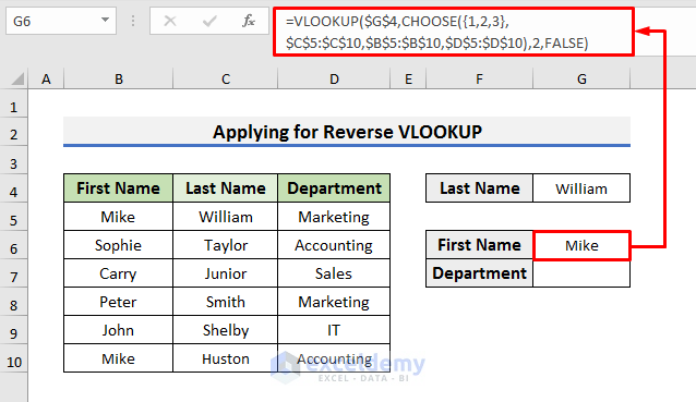
- First of all, to get the First Name, select Cell G6 and type the formula below:
- Now, press Enter to see the result.
In this formula, the CHOOSE function creates a new table or array that stores the Last Name as the leftmost column, the First Name as the middle column, and the Department as the third column. The VLOOKUP formula looks for the value of Cell G4 in the new table and returns the desired value from the second column of that table.
- Similarly, use the formula below in Cell G7 to get the Department of the employee:
7. Generate Random Data Using Excel CHOOSE Function
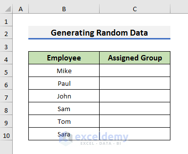
In this example, we will apply the CHOOSE function to assign groups to some employees for completing different tasks. But interestingly, we want to assign the groups randomly. For that purpose, we can use the RANDBETWEEN function. The RANDBETWEEN function returns a series of numbers from the specified range of numbers.
Let’s follow the steps below to assign groups randomly.
STEPS:
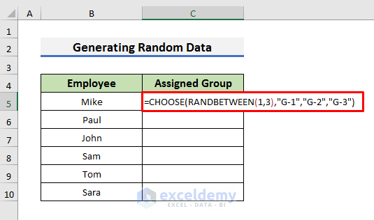
- To begin with, select Cell C5 and type the formula below:
In this formula, the RANDBETWEEN function generates a random number from 1 to 3 as the index number of the CHOOSE function. Based on the index number, the CHOOSE function selects a group from the list.
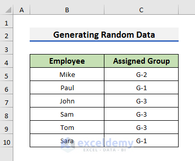
- In the following step, press Enter and drag down the Fill Handle to copy the formula to Cell C10.
Note: The RANDBETWEEN function is a volatile function. So, if you make any changes on the sheet, the assigned groups will automatically change. To make the assigned groups hard-coded, you can paste the values after getting the groups.
Read More: How to Use RANDBETWEEN with CHOOSE Function in Excel
8. Create Formula with CHOOSE Function to Return Next Working Day
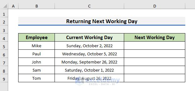
Another advanced application of the CHOOSE function in Excel is to return the working day. To do so, we need to know the current working day. We will use the dataset below to explain the example. You can see the different current working days of some employees. We will find the next working day using the WEEKDAY function with the CHOOSE function.
Let’s pay attention to the steps below to learn more.
STEPS:
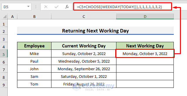
- In the beginning, select Cell D5 and type the formula below:
- Press Enter.
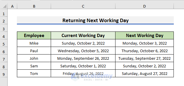
The formula may look complex at the first glance. Here, we are adding the value that the CHOOSE function returns with Cell C5. The WEEKDAY function returns a number as the index number of today’s date. Depending on the index number, the CHOOSE function selects a value from the list {1,1,1,1,1,3,2}. And then the addition happens.
- After that, drag the Fill Handle down to copy the formula.
9. Get Total Sales for Specific Store with Excel CHOOSE Function
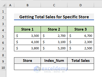
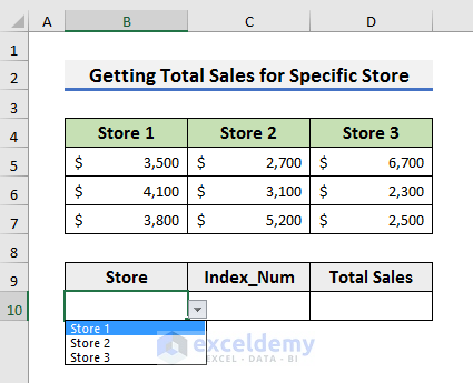
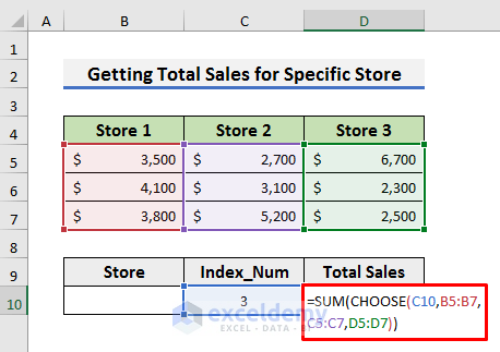
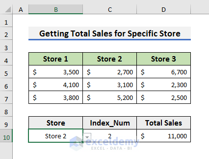
This example is similar to Example 3 but it is another advanced application of the CHOOSE function. Here, we will try to get the total sales for a specific store with the CHOOSE function in Excel. We will select the store using a drop-down list and the total sales of that store will be visible in Cell D10.
Let’s follow the steps to learn the whole application.
STEPS:
- Firstly, select Cell B10.
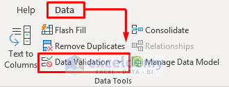
- Then, go to the Data tab and select Data Validation. It will open the Data Validation box.
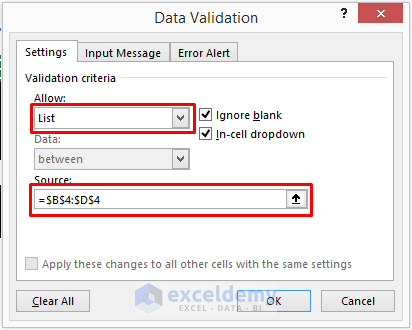
- Select List in the Allow field.
- After that, enable editing in the Source field and select the range B4:B7.
- Click OK to proceed.
- You can now choose the store from the drop-down list.
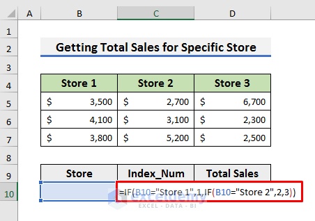
- In the following step, select Cell C10 and type the formula below:
- Press Enter.
Here, we have used the Nested IFs to assign index numbers for each store. This formula states that if Cell B10 contains Store 1, then it will print 1. If it contains Store 2, then it will show 2. Otherwise, it will print 3.
- Now, select Cell D10 and type the formula below:
- Hit Enter.
We have explained the same formula in Example 3.
- Finally, if you select Store 2 using the drop-down list, you will find the total sales in Cell D10.
Read More: How to Apply CHOOSE Function to Create Drop-Down List in Excel
Conclusion
In this article, we have 9 advanced and useful applications of Excel CHOOSE Function. I hope this article will help you to perform your tasks efficiently. Furthermore, we have also added the practice book at the beginning of the article. To test your skills, you can download it to exercise. Also, you can visit the ExcelDemy website for more articles like this. Lastly, if you have any suggestions or queries, feel free to ask in the comment section below.
ليست هناك تعليقات:
إرسال تعليق