Statistical Functions(SUM, COUNT, and AVERAGE Functions)

 

Statistical Functions(SUM, COUNT, and AVERAGE Functions)

So far, our formulas have only referenced individual cells. Formulas can also be used

to perform calculations on entire ranges of cells. To add a series of cells, you could type:

=a1+a1+a3+a4+a5

However, that is not feasible when working with large data sets. Instead you should use the SUM Function:

=sum(a1:a5)

This will sum the entire range from A1 to A5. Notice how the range is entered using a colon (:) to separate the first and last cells in the range. Instead of typing the range, you could also select your range of cells using the keyboard: Hold down SHIFT while using the Arrow Keys. If you are not familiar with how to use the keyboard to navigate and select cells, we recommend going through our Keyboard Shortcut App

Now practice with the AVERAGE Function.

1. Average range B3 to B6.(Hint)

Save Question to Custom Practice Set?

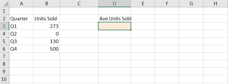
The SUM, COUNT, and AVERAGE Functions will ignore cells that contain text, numbers stored as text, or blank values. They will only include cells with valid numbers.

In order to accommodate different scenarios, Excel provides several variations of these basic functions:

Average	Count	Sum	Description
Average	Count	Sum	Skips Blanks and Text
AverageA	CountA		Skips Blanks, Includes Text
	CountBlank		Count Blanks Only

2. Count the number of blank cells in range B3 to B6 using COUNTBLANK.(Hint)

Save Question to Custom Practice Set?

3. Count all non-blank cells in range B3 to B6.(Hint)

Save Question to Custom Practice Set?

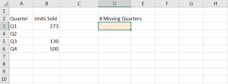
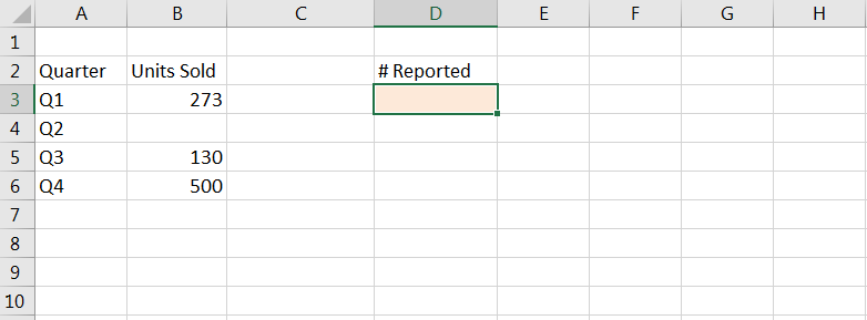
SUMIFs, COUNTIFs, and AVERAGEIFs Functions

These functions are some of the most powerful functions in Excel. They allow you to sum, count, or average only the cells within a range that meet certain criteria.

Function	Syntax
Countifs	=countifs(criteria_range1, criteria, ...)
Averaageifs	=averageifs(average_range, criteria_range1, criteria, ...)
Sumifs	=sumifs(sum_range, criteria_range1, criteria, ...)

Notice how the Countif function is slightly different? It does not require a "count_range" because it does not need a range to calculate, it only needs to count the number of times the criteria is met.

Examples:

Average all Q1 Sales:

=SUMIFS(J3:J14,I3:I14,1)

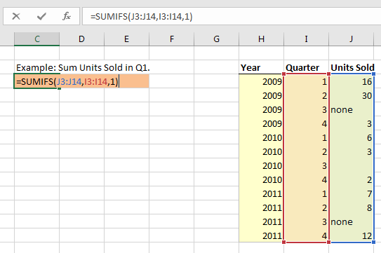
Here we defined the criteria_range as “Quarter” and the sum_range as “Units Sold”. Note: in our example we excluded the $-signs for locking cell references. We did this so that the formulas are easier to follow. Generally, with formulas like these you would want to lock cell references:

=SUMIFS($J$3:$J$14$,$I3:$I$14,1)

Now we will look at an example with more than one criteria

Count the number of quarters after 2009 with more than 5 units sold:

=COUNTIFS(J3:J14,">5",H3:H14,">2009")

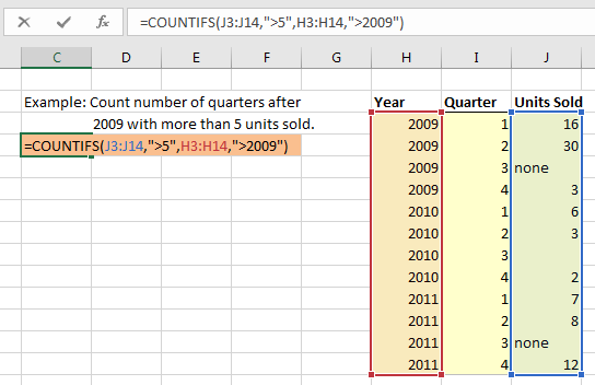
Notice that with the COUNTIFS Function we do not need to define a “count_range”. Also, notice how we entered the criteria. We will review this in more detail next.

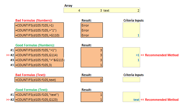
"IFs" Criteria

When first using these functions, it can be very frustrating to understand how to enter the proper criteria. Essentially, the criteria must be a string of text. Remember that! Whenever you enter criteria for these functions, think about creating a text string! Now we will review some examples:

To enter an exact match directly into the function:

“Q1”

To enter a comparison directly into the function:

“<0”

to Enter the criteria into a cell and reference the criteria (note: the criteria can be an exact match or a string of text representing a comparison.):

a1

To Use a combination:

”<” & a1

Note: In the last example we use the & character to combine two strings of text. We will learn more about that in the Text Functions section.

Here are more examples of good and bad COUNTIFS Functions:

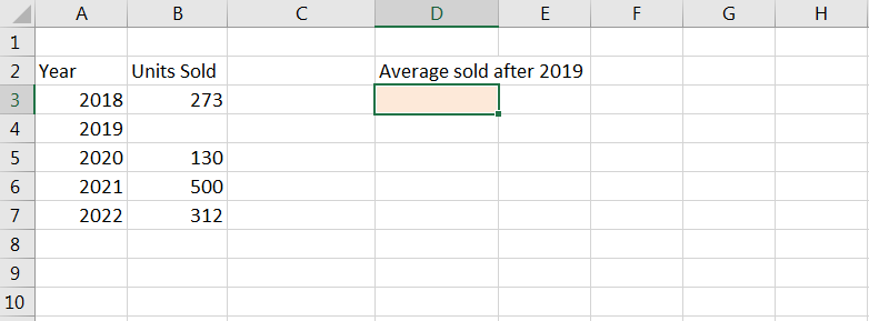
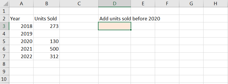
Now, it is your turn!

4. Average the units sold after 2019(Hint)

Save Question to Custom Practice Set?

5. Count the number of years after 2019 with less than 300 units sold.(Hint)

Save Question to Custom Practice Set?

6. Add together the Units sold before 2020.(Hint)

Save Question to Custom Practice Set?

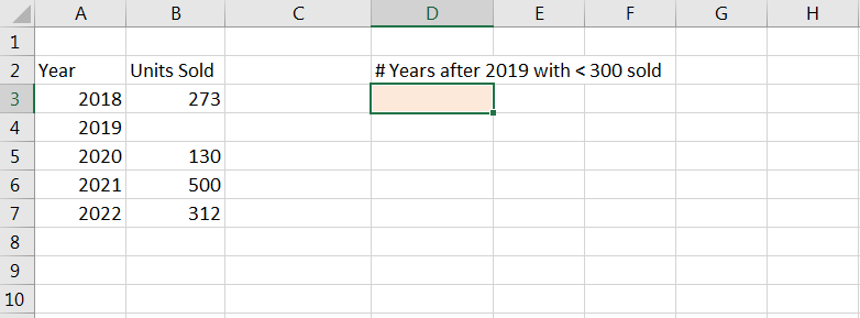
Wildcards

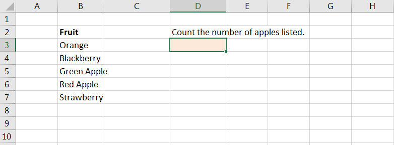
Wildcards are characters that can be used for “inexact” matches. They can be used in the previous SUMIFS, COUNTIFS, AVERAGEIFS Functions, lookup functions (ex. VLOOKUP), Find, Autofilter, and much more.

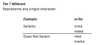
The ? Wildcard represents any single character:

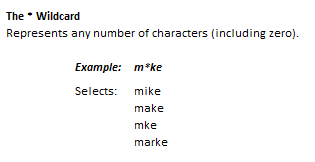
The * Wildcard represents any number of characters (including 0)

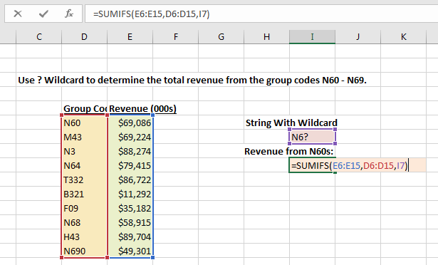
Use the Wildcards exactly like any other text character. Instead of typing “t” for “t”, type “?” for any single character or “*” for any number of any character.

Example:

7. Using a wildcard, create a COUNTIFs formula in cell C4 that will count the total number of apples (of all types).(Hint)

Save Question to Custom Practice Set?

Sumproduct Function

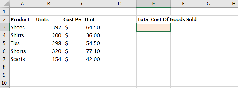
The SUMPRODUCT Functions adds together the products of parallel arrays of cells. It is easier to explain with an example:

In this example, our goal is to calculate total sales revenue. We could create an additional column, multiply each row (Units Sold * Price Per Unit), and add together the results. Or we could use a single SUMPRODUCT formula to perform the same calculation using a single cell.

8. Using SUMPRODUCT, calculate the total cost of goods sold (sum the product of each unit # * cost per unit).(Hint)