مكافآة نهاية الخدمة وفقاً لقانون العمل المصري رقم 12 لسنة 2003م وتعديلاته.

 

مكافآة نهاية الخدمة وفقاً لقانون العمل المصري رقم 12 لسنة 2003م وتعديلاته.

Excel Shortcuts List جميع اختصارات الاكسل

 

Excel Shortcuts List جميع اختصارات الاكسل 

How to Use this Shortcut List:

+ Indicates to hold the previous key, while pressing the next key.

> Indicates to tap the previous key, releasing it before pressing the next key.

Find the shortcuts li

Date Functions

 

Date Formulas

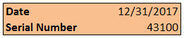
The most important thing to understand about dates is that Excel stores dates as serial numbers. The serial number represents the number of days from (the imaginary) day of 1/0/1900.

Text Functions

 

Text Formula Basics

If you have made it this far, you know that any time you use text in a formula, you must surround the text with quotations.

Lookup Functions

 

VLOOKUP Functions

The VLOOKUP Function might be the most talked about Excel function. Job interviewers ask candidates to explain how it works. It is the function that weeds out Excel wannabes. If you want to become competent in Excel you must master this function.

VLOOKUPs allow you to “lookup” a value in a data set and return information from the row where that value 

Statistical Functions(SUM, COUNT, and AVERAGE Functions)

 

Statistical Functions(SUM, COUNT, and AVERAGE Functions)

So far, our formulas have only referenced individual cells. Formulas can also be used

Logical Functions

 

Logical Functions

C

Excel Functions List جميع دوال الاكسل المهمه

 

Excel Functions List جميع دوال الاكسل المهمه

Below you will find a searchable list of ~200 Excel Functions. Next to each function, you'll see a description of the function along with the function's syntax.

If you'd like to learn more about a function, simply click it's row and go to the function page. Each function page contains detailed instructions on how to use the function, including multiple examples.

We also recommend checking out our Formula Examples Page. This page contains 100 (and growing rapidly) formula examples for specific use-cases (ex. count all cells with positive numbers)

 

Searchable Drop-Down Lists in Excel with ZERO Effort

FINALLY!!!

Excel now supports searchable drop-down lists!

Until this new feature hit the streets, searchable drop-down lists required writing complex VBA code coupled with advanced Excel features to work properly.

Searchable drop-down lists now work without any user effort whatsoever.  The feature is native to Excel.

In January 2022, this feature is available to select Beta Channel users of Office 365.  When officially released, the feature will be rolled out to Office 365 and standalone Excel users running the latest yearly version

Let’s look at an example of this wonderful, soon-to-be-released, new feature.

Excel LAMBDAs

 

Excel LAMBDAs Made Easy with the New Advanced Formula Environment (Editor)

Microsoft has released a new, official add-in for Excel called the “Advanced Formula Editor”.

If you have used Excel’s Name Manager to create more complex formulas that can be referenced via a single word, you no doubt experienced the pain associated with a decade’s old interface.

As Excel has evolved over the years, the Name Manager’s interface has not changed to keep up with the new demands placed upon it.

Let’s examine Excel’s new kid on the block for managing complex formulas with assigned names, the Advanced Formula Environment (Editor).

 

Excel’s VSTACK – The One Function to Append Them All

Imagine a workbook with 12 sheets containing sales tables: January through December.

Now imagine a workbook with 50 sheets containing product distribution tables: Alabama through Wyoming.

Brace yourself.  Now imagine a workbook with 195 sheets containing gross domestic product tables: Afghanistan through Zimbabwe.

Which do you think would be easier to combine into a single table, the file with 12, 50, or 195 sheets?

It’s a trick question.  They all take the same amount of effort provided you use the correct Excel feature.

Let’s examine how we can accomplish this using a single formula.  Yes, you read that correctly, a single formula.

 

Excel VBA vs Office Scripts

Do you need to switch?

If you have used macros in Excel you know that they can save you a tremendous amount of time when performing common tasks along with greatly improving the accuracy of your workflows.

Simple macros (defined as macros with basic, linear process flows) can be easily created using the macro Recorder.  More complex macros, like those that may solicit the user for input, contain branching logic, or perform error checking need to be written by hand inside the macro code editor.

Macros are written in a language called Visual Basic for Applications, or VBA for short, which is a subset of Visual Basic.

How do Office Scripts fit into this workflow automation scheme?  What are some of the differences between VBA macros and Office Scripts?  Are Office Scripts the successor to VBA macros?

Let’s look at the facts and see if this New Kid on the Block is here to dethrone Old Faithful.

Yearly Calendar with a Formula in Excel and Sheets

 Yearly Calendar with a Formula in Excel and Sheets

To make our interactive yearly calendar as seen above, we will take advantage of one of the new 

Excel Dynamic Array functions called SEQUENCE.

User Input and Formula Output

The goal is to have the user type a year in a cell, such as D2, and have the SEQUENCE function generate all the calendar dates for that year, structured in a 7-day by 54-week table.

NOTE: We require a 54-week table because of an oddity that occurs every 28 years.  Using the year 2000 as an easy start, the month of July has 6 weeks. This adds an extra week to the more common 53-week year.  Every 28 years before and after the year 2000 have this same 

the FILTER function) FILTER(array, include, [if_empty])

 

To understand the FILTER function, the syntax is as follows (parameters in brackets are optional):

FILTER(array, include, [if_empty])

• array – is the range or array you want to be included in the result. This can be the entire data set or part of the original data set.

• include – is the test you are performing on each record in the data set. This is the engine that moves the FILTER function forward.  Here is where you define the criteria for included versus excluded records.
  The logic will resemble the test portion of an IF function; we select a range of cells and compare each item in the range to a defined value (ex: B8:B40=E6, where column B is the data and cell E6 is what the data is being compared against.)  Any record that results in a TRUE statement will be included in the results.  Any record that results in a FALSE statement will be excluded from the results.

• [if_empty] – defines what is to be displayed if no records match the include test (ex: “No Data”). Although this argument is optional, if it is not defined, and no data is returned from the include test, a #CALC! error will be displayed.

The LET function

 

LET Function Syntax

The LET function has the following syntax:

=LET(name1, name_value1, calculation_or_name2, [name_value2, calculation_or_name3…] )

• name1: is the first name to assign and must begin with a letter. This cannot be the output of a formula or refer to an existing named range.
• name_value1: is the value assigned to the name1
• calculation_or_name2: can be a calculation that uses all names within the LET function or a second name assigned to the name_value2 If this is the latter, then the calculation_or_name3 argument becomes required.
• name_value2: (optional) is the value assigned to the calculation_or_name2
• calculation_or_name3: (optional) can be a calculation that uses all names within the LET function or a second name assigned to the name_value2 If this is the latter, then the calculation_or_name4 argument becomes required.

Excel XLOOKUP

 

Excel XLOOKUP Explained

(Goodbye VLOOKUP!)

In this post, we will examine Excel’s BEST function for performing a lookup…

We’re going to look at how the new (upcoming) XLOOKUP function solves common lookup problems typically solved by older functions like…

• LOOKUP
• VLOOKUP
• HLOOKUP
• INDEX/MATCH

This will be just a glimpse of some of the many and varied uses of the XLOOKUP function.  We will explore many more uses of XLOOKUP in future videos.

Our Lookup Challenge

We have a dataset that contains information about an employee’s start date within a Division and Department.  This is on a sheet named “MD” for “Master Data”.

We would like to find an employee name from the list below and return the Division that the user was originally assigned and place the result in Column C.

We would also like to calculate the employee’s Bonus based on the Yearly Sales (Column B) and place the results in Column E.

The calculations for the Bonus are based on the following table.

Basic Lookup

Let’s begin by looking up the user’s Division.  We’ll select the first empty cell below our Division heading and enter the following formula.

=XLOOKUP(A5, MD!$D$5:$D$37, MD!$B$5:$B$37)

The logic works like so:

=XLOOKUP(lookup_value, lookup_array, return_array)

NOTE:  There are three additional optional arguments that we will examine later in the post.

• lookup_value – is the value we want to find (cell A5)
• lookup_array – is the list to find the lookup_value in (sheet “MD” cells D5:D37)
• return_array – is the list to return from upon discovery (sheet “MD” cells B5:B37)

We have “locked” the references to the lookup_array ($D$5:$D$37) and return_array ($B$5:$B$37) since we want those references to remain the same when we fill the formula down the list of names.

If you don’t want to deal with relative/absolute references, consider converting the data to a proper Excel Table to use structured references instead of traditional cell references.

Notice that we didn’t have to tell XLOOKUP to perform an exact match lookup because XLOOKUP defaults to exact match.  Unlike VLOOKUP/HLOOKUP where you had to expressly tell them to perform an exact match, we don’t need to define anything for this behavior.

Fill the XLOOKUP formula down the list to see the results.

Did you see the hidden awesomeness?

Notice that in the data, the column that we are returning data from is to the LEFT of the column we are searching.

This would be impossible with a traditional VLOOKUP function (without performing some crazy in-memory, virtual table construction which only 9 people on planet Earth find enjoyable.)

Finding the LATEST Division Assignment

Notice in the Division results column, we have identified “Kim West” as being a member of the “Utility” Division.

If we look at the data, we see that “Kim West” appears twice.

This is because “Kim” was originally assigned to the “Utility” Division upon initial hiring but was then transferred to the “Game” Division a few years later.

Like the VLOOKUP function, XLOOKUP returned the Division for the first discovered instance of “Kim West” in the Name column.

What if we need to return the LAST assigned Division?

Discover the Last Match

Since our data is sorted in ascending order by Start Date, we can use an optional argument to perform a “reverse lookup” so we stop on the last instance of “Kim West” (we’re actually stopping on the first encountered item in the list when you search from the bottom-up.)

We will copy the formula we used to discover Division and paste it below the Current Division heading.  The formula requires the following modification:

=XLOOKUP(A5, MD!$D$5:$D$37, MD!$B$5:$B$37, "Not Found", 0, -1)

The logic of the additional arguments works like so:

=XLOOKUP(lookup_value, lookup_array, return_array, [if_not_found], [match_mode], [search_mode])

NOTE:  The two additional arguments are optional, hence the square brackets.

• [if_not_found] – is what to display if no match exists (e. text message or default value)
• [match_mode] – specifies the Match Type. (0 = Exact match {default}, -1 = Exact match or next smaller, 1 = Exact match or next larger, 2 = Wildcard match)
• [search_mode] – specifies the Search Mode. (1 = Search first to last {default}, -1 = Search last to first, 2 = Binary search {ascending}, -2 = Binary search {descending})

In our case, we are performing an exact match (0) from the last record to the first record (-1) and we will display a message (“Not Found”) if there is not a match .

We see that “Kim West” began her employment working in the “Utility” Division, but currently resides in the “Game” Division.

Get the Next Smallest Value

Next, we will discover the Bonus amount based on the value in the Yearly Salary column.

The Yearly Salary will be located in the following table and once found, will return the Bonus percentage.

Since the table establishes ranges of salaries, the odds are slim that we will search for a value that is defined in the Salary column.  Instead, we will need to return the Bonus for the Salary that is the closest without going over.

Select the first empty cell below our Bonus heading and enter the following formula.

=XLOOKUP(B5, MD!$G$5:$G$9, MD!$H$5:$H$9, "Not Found", -1)

The results are as follows.

“Kim West” has a yearly salary of 60,200.  The closest value to 60,200 without going over is $60,000.  Therefore, we return 10%.

Remember, the -1 in the [match_mode] argument means “exact match or next smaller item”.

XLOOKUP – Super Amazing Feature

In the previous example, we searched for the value “closest to without going over” our lookup value.  The table was sorted from the smallest value to the largest value, as all lookup tables are required to be when performing an approximate match lookup.

Check THIS out!  We can list the salaries in any order we want… AND IT STILL WORKS!!!

This means you can sort your lists ANY WAY YOU WISH, and the lookup still works.

Not So Final Thoughts

There is a tremendous amount of potential lurking behind the new XLOOKUP function.  This tutorial hasn’t even scratched the surface when it comes to demonstrating XLOOKUP’s potential.

We will explore many other ways to use XLOOKUP in future tutorials.  For now, give it a try and be amazed.