شرح دالة filter مع الامثلة

 

شرح دالة filter  مع الامثلة

Excel FILTER function

The FILTER function in Excel is used to filter a range of data based on the criteria that you specify.

The function belongs to the category of Dynamic Arrays functions. The result is an array of values that automatically spills into a range of cells, starting from the cell where you enter a formula.

The syntax of the FILTER function is as follows:

FILTER(array, include, [if_empty])

Where:

• Array (required) - the range or array of values that you want to filter.
• Include (required) - the criteria supplied as a Boolean array (TRUE and FALSE values).
  Its height (when data is in columns) or width (when data is in rows) must be equal to the that of the array argument.
• If_empty (optional) - the value to return when no entries meet the criteria.

The FILTER function is only available in Excel for Microsoft 365 and Excel 2021. In Excel 2019, Excel 2016 and earlier versions, it is not supported.

Basic Excel FILTER formula

For starters, let's discuss a couple of very simple cases just to gain more understanding how an Excel formula to filter data works.

From the below data set, supposing you want to extract the records with a specific value in the Group, column, say group C. To have it done, we supply the expression B2:B13="C" to the include argument, which will produce a required Boolean array, with TRUE corresponding to "C" values.

=FILTER(A2:C13, B2:B13="C", "No results")

In practice, it's more convenient to input the criteria in a separate cell, e.g. F1, and use a cell reference instead of hardcoding the value directly in the formula:

=FILTER(A2:C13, B2:B13=F1, "No results")

Unlike Excel's Filter feature, the function does not make any changes to the original data. It extracts the filtered records into the so-called spill range (E4:G7 in the screenshot below), beginning in the cell where the formula is entered: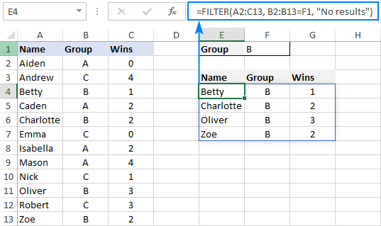

If no records match the specified criteria, the formula returns the value you put in the if_empty argument, "No results" in this example: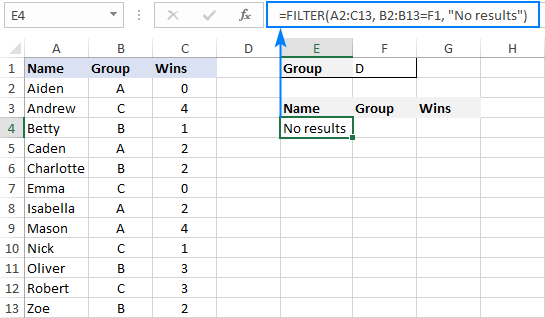

If you'd rather return nothing in this case, then supply an empty string ("") for the last argument:

=FILTER(A2:C13, B2:B13=F1, "")

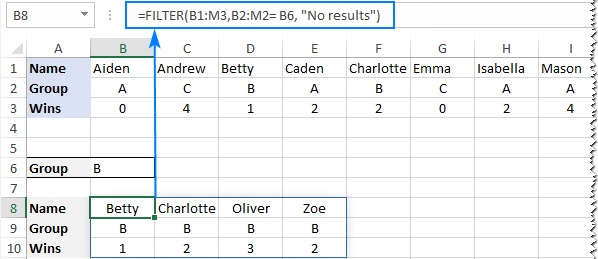
In case your data is organized horizontally from left to right like shown in the screenshot below, the FILTER function will work nicely too. Just make sure you define appropriate ranges for the array and include arguments, so that the source array and Boolean array have the same width:

=FILTER(B2:M4, B3:M3= B7, "No results")

Excel FILTER function - usage notes

To effectively filter in Excel with formulas, here are a couple of important points to take notice of:

• The FILTER function automatically spills the results vertically or horizontally in the worksheet, depending on how your original data is organized. So, please make sure you always have enough empty cells down and to the right, otherwise you'll get a #SPILL error.
• The results of the Excel FILTER function are dynamic, meaning they update automatically when values in the original data set change. However, the range supplied for the array argument is not updated when new entries are added to the source data. If you wish the array to resize automatically, then convert it to an Excel table and build formulas with structured references, or create a dynamic named range.

How to filter in Excel - formula examples

Now that you know how a basic Excel filter formula works, it's time to get some insights into how it could be extended for solving more complex tasks.

Filter with multiple criteria (AND logic)

To filter data with multiple criteria, you supply two or more logical expressions for the include argument:

FILTER(array, (range1=criteria1) * (range2=criteria2), "No results")

The multiplication operation processes the arrays with the AND logic, ensuring that only the records that meet all the criteria are returned. Technically, it works this way:

The result of each logical expression is an array of Boolean values, where TRUE equates to 1 and FALSE to 0. Then, the elements of all the arrays in the same positions are multiplied. Since multiplying by zero always gives zero, only the items for which all the criteria are TRUE get into the resulting array, and consequently only those items are extracted.

The below examples show this generic formula in action.

Example 1. Filter multiple columns in Excel

Extending our basic Excel FILTER formula a little further, let's filter the data by two columns: Group (column B) and Wins (column C).

For this, we set up the following criteria: type the name of the target group in F2 (criteria1) and the minimum required number of wins in F3 (criteria2).

Given that our source data is in A2:C13 (array), groups are in B2:B13 (range1) and wins are in C2:C13 (range2), the formula takes this form:

=FILTER(A2:C13, (B2:B13=F2) * (C2:C13>=F3), "No results")

As the result, you get a list of players in group A who have secured 2 or more wins: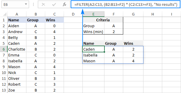

Example 2. Filter data between dates

First off, it should be noted that it's not possible to make up a generic formula to filter by date in Excel. In different situations, you will need to build criteria differently, depending on whether you want to filter by a specific date, by month, or by year. The purpose of this example is to demonstrate the general approach.

To our sample data, we add one more column containing the dates of the last win (column D). And now, we will extract the wins that occurred in a specific period, say between May 17 and May 31.

Please notice that in this case, both criteria apply to the same range:

=FILTER(A2:D13, (D2:D13>=G2) * (D2:D13<=G3), "No results")

Where G2 and G3 are the dates to filter between.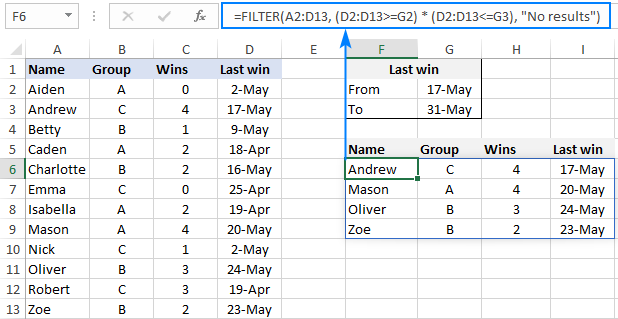

Filter with multiple criteria (OR logic)

To extract data based on multiple OR condition, you also use logical expressions like shown in the previous examples, but instead of multiplying, you add them up. When the Boolean arrays returned by the expressions are summed, the resulting array will have 0 for entries that do not meet any criteria (i.e. all the criteria are FALSE), and such entries will be filtered out. The entries for which at least one criterion is TRUE will be extracted.

Here's the generic formula to filter columns with the OR logic:

FILTER(array, (range1=criteria1) + (range2=criteria2), "No results")

As an example, let's extract a list of players that have this or that number of wins.

Assuming the source data is in A2:C13, wins are in C2:C13, and the win numbers of interest are in F2 and F3, the formula would go as follows:

=FILTER(A2:C13, (C2:C13=F2) + (C2:C13=F3), "No results")

As the result, you know which players have won all the games (4) and which have won none (0):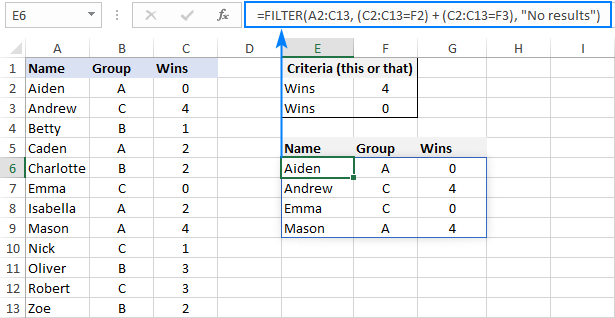

Filter based on multiple AND as well as OR criteria

In situation when you need to apply both criteria types, remember this simple rule: join the AND criteria with asterisk (*) and OR criteria with the plus sign (+).

For example, to return a list of players that have a given number of wins (F2) AND belong to the group mentioned in either E2 OR E3, build the following chain of logical expressions:

=FILTER(A2:C13, (C2:C13=F2) * ((B2:B13=E2) + (B2:B13=E3)), "No results")

And you will get the following result: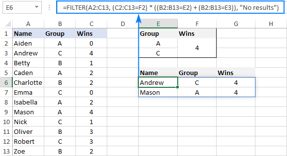

How to filter duplicates in Excel

When working with huge worksheets or combining data from different sources, there's often a possibility that some duplicates would sneak in.

If you are looking to filter out duplicates and extract unique items, then use the UNIQUE function as explained in the above linked tutorial.

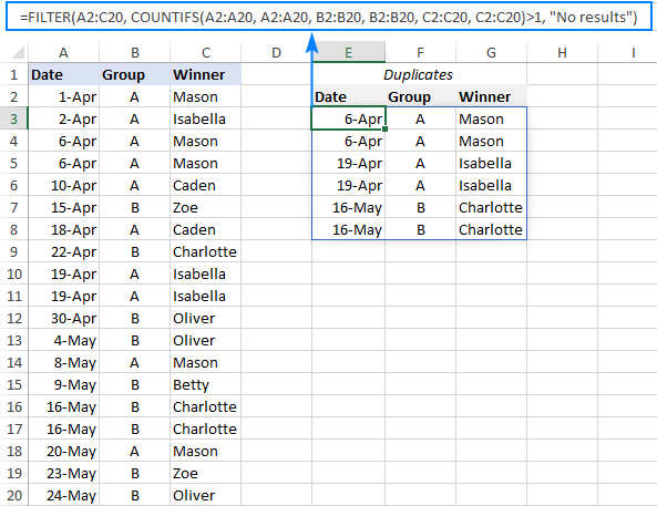
If your goal is to filter duplicates, i.e. extract entries that occur more than once, then use the FILTER function together with COUNTIFS.

The idea is to get the occurrences counts for all the records and extract those greater than 1. To get the counts, you supply the same range for each criteria_range / criteria pair of COUNTIFS like this:

FILTER(array, COUNTIFS(column1, column1, column2, column2)>1, "No results")

For example, to filter duplicate rows from the data in A2:C20 based on the values in all 3 columns, here's the formula to use:

=FILTER(A2:C20, COUNTIFS(A2:A20, A2:A20, B2:B20, B2:B20, C2:C20, C2:C20)>1, "No results")

Tip. To filter duplicates based on the values in the key columns, include only those specific columns in the COUNTIFS function.

How to filter out blanks in Excel

A formula for filtering out blank cells is, in fact, a variation of the Excel FILTER formula with multiple AND criteria. In this case, we check whether all (or particular) columns have any data in them and exclude the rows where at least one cell is empty. To identify non-blank cells, you use the "not equal to" operator (<>) together with an empty string ("") like this:

FILTER(array, (column1<>"") * (column2=<>""), "No results")

With the source data in A2:C12, to filter out rows containing one or more blank cells, the following formula is entered in E3: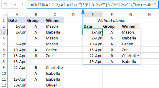

Filter cells containing specific text

To extract cells that contain certain text, you can use the FILTER function together with the classic If cell contains formula:

FILTER(array, ISNUMBER(SEARCH("text", range)), "No results")

Here's how it works:

• The SEARCH function looks for a specified text string in a given range and returns either a number (the position of the first character) or #VALUE! error (text not found).
• The ISNUMBER function converts all the numbers to TRUE and errors to FALSE and passes the resulting Boolean array to the include argument of the FILTER function.

For this example, we've added the Last names of players in B2:B13, typed the part of the name we want to find in G2, and then use the following formula to filter the data:

=FILTER(A2:D13, ISNUMBER(SEARCH(G2, B2:B13)), "No results")

As the result, the formula retrieves the two surnames containing "han":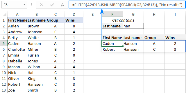

Filter and calculate (Sum, Average, Min, Max, etc.)

A cool thing about the Excel FILTER function is that it can not only extract values with conditions, but also summarize the filtered data. For this, combine FILTER with aggregation functions such as SUM, AVERAGE, COUNT, MAX or MIN.

For instance, to aggregate data for a specific group in F1, use the following formulas:

Total wins:

=SUM(FILTER(C2:C13, B2:B13=F1, 0))

Average wins:

=AVERAGE(FILTER(C2:C13, B2:B13=F1, 0))

Maximum wins:

=MAX(FILTER(C2:C13, B2:B13=F1, 0))

Minimum wins:

=MIN(FILTER(C2:C13, B2:B13=F1, 0))

Please pay attention that, in all the formulas, we use zero for the if_empty argument, so the formulas would return 0 if no values meeting the criteria are found. Supplying any text such as “No results” would result in a #VALUE error, which is obviously the last thing you want :)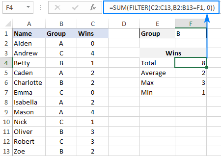

Case-sensitive FILTER formula

A standard Excel FILTER formula is case-insensitive, meaning it makes no distinction between lowercase and uppercase characters. To distinguish text case, nest the EXACT function in the include argument. This will force FILTER to do logical test in a case-sensitive manner:

FILTER(array, EXACT(range, criteria), "No results")

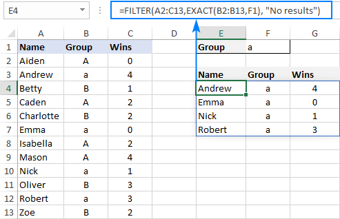
Supposing, you have both groups A and a and wish to extract records where the group is the lowercase "a". To have it done, use the following formula, where A2:C13 is the source data and B2:B13 are groups to filter:

=FILTER(A2:C13, EXACT(B2:B13, "a"), "No results")

As usual, you can input the target group in a predefined cell, say F1, and use that cell reference instead of hardcoded text:

=FILTER(A2:C13, EXACT(B2:B13, F1), "No results")

How to FILTER data and return only specific columns

For the most part, filtering all columns with a single formula is what Excel users want. But if your source table contains tens or even hundreds of columns, you may certainly want to limit the results to a few most important ones.

Example 1. Filter some adjacent columns

In situation when you want some neighboring columns to appear in a FILTER result, include only those columns in array because it is this argument that determines which columns to return.

In the basic FILTER formula example, supposing you wish to return the first 2 columns (Name and Group). So, you supply A2:B13 for the array argument:

=FILTER(A2:B13, B2:B13=F1, "No results")

As the result, we get a list of participants of the target group defined in F1:

Example 2. Filter non-adjacent columns

To cause the FILTER function to return non-contiguous columns, use this clever trick:

1. Make a FILTER formula with the desired condition(s) using the entire table for array.
2. Nest the above formula inside another FILTER function. To configure the "wrapper" function, use an array constant of TRUE and FALSE values or 1's and 0's for the include argument, where TRUE (1) marks the columns to be kept and FALSE (0) marks the columns to be excluded.

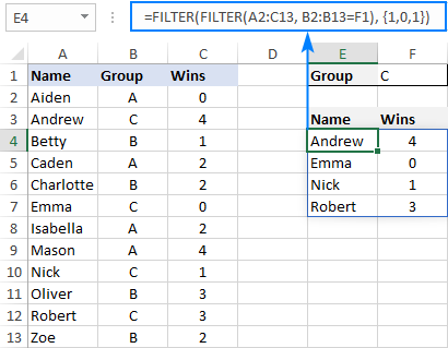
For example, to return only Names (1^st column) and Wins (3^rd column), we are using {1,0,1} or {TRUE,FALSE,TRUE} for the include argument of the outer FILTER function:

=FILTER(FILTER(A2:C13, B2:B13=F1), {1,0,1})

Or

=FILTER(FILTER(A2:C13, B2:B13=F1), {TRUE,FALSE,TRUE})

How to limit the number of rows returned by FILTER function

If your FILTER formula finds quite a lot of results, but your worksheet has limited space and you cannot delete the data below, then you can limit the number of rows the FILTER function returns.

Let's see how it works on an example of a simple formula that pulls players from the target group in F1:

=FILTER(A2:C13, B2:B13=F1)

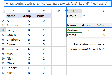
The above formula outputs all the records that it finds, 4 rows in our case. But suppose you just have space for two. To output only the first 2 found rows, this is what you need to do:

• Plug the FILTER formula into the array argument of the INDEX function.
• For the row_num argument of INDEX, use a vertical array constant like {1;2}. It determines how many rows to return (2 in our case).
• For the column_num argument, use a horizontal array constant like {1,2,3}. It specifies which columns to return (the first 3 columns in this example).
• To take care of possible errors when no data matching your criteria is found, you can wrap your formula in the IFERROR function.

The complete formula takes this form:

=IFERROR(INDEX(FILTER(A2:C13, B2:B13=F1), {1;2}, {1,2,3}), "No result")

When working with large tables, writing array constants manually may be quite cumbersome. No problem, the SEQUENCE function can generate the sequential numbers for you automatically:

=IFERROR(INDEX(FILTER(A2:C13, B2:B13=F1), SEQUENCE(2), SEQUENCE(1, COLUMNS(A2:C13))), "No result")

The first SEQUENCE generates a vertical array containing as many sequential numbers as specified in the first (and only) argument. The second SEQUENCE uses the COLUMNS function to count the number of columns in the dataset and produces an equivalent horizontal array.

Tip. To return data from specific columns, not all the columns, in the horizontal array constant that you use for the column_num argument of INDEX, include only those specific numbers. For instance, to extract data from the 1st and 3rd columns, use {1,3}.

Excel FILTER function not working

In situation when your Excel FILTER formula results in an error, most likely that will be one of the following:

#CALC! error

Occurs if the optional if_empty argument is omitted, and no results meeting the criteria are found. The reason is that currently Excel does not support empty arrays. To prevent such errors, be sure to always define the if_empty value in your formulas.

#VALUE error

Occurs when the array and include argument have incompatible dimensions.

#N/A, #VALUE, etc.

Different errors may occur if some value in the include argument is an error or cannot be converted to a Boolean value.

#NAME error

Occurs when trying to use FILTER in an older version of Excel. Please remember that it is a new function, which is only available in Office 365 and Excel 2021.

In new Excel, a #NAME error occurs if you accidentally misspell the function's name.

#SPILL error

Most often, this error occurs if one or more cells in the spill range are not completely blank. To fix it, just clear or delete non-empty cells. To investigate and resolve other cases, please see #SPILL! error in Excel: what it means and how to fix.

#REF! error

Occurs when a FILTER formula is used between different workbooks, and the source workbook is closed.

That's how to filer data in Excel dynamically. I thank you for reading and hope to see you on our blog next week!